The ONL Tutorial

Tutorial >> The Remote Laboratory Interface

TOC

Monitoring Concepts

The ONL routers maintain numerous monitoring points (places with counters). Some of these are inside the FPX port processors, and some are actually inside the ATM switch port processors. The ubiquity of monitoring points makes it easy to observe traffic in places not often available in other systems. The downside is that sometimes measurements can be misinterpreted unless you pay attention to the measurement details. This page explains how monitored parameters are computed.

What Was Monitored In The Ping Example?

In the ping traffic example described in the Basic Monitoring page, the bandwidth plots were derived from reading ATM cell and and timestamp counters inside the ATM switch rather than at the FPX port processors. These four monitoring points inside of NSP 1 are shown in Fig. 1 as solid red dots labeled A, B, C and D. The red arrows indicate the two paths through NSP 1 of the ICMP echo request packets and returning the ICMP echo reply packets.

Fig. 1. Ping Traffic Monitoring Points.

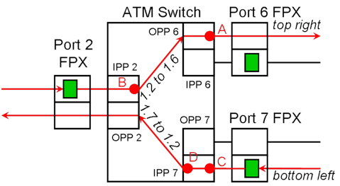
At the center is the ATM switch that carries the traffic from ingress (input) side to egress (output) side. Each port of the ATM switch contains a pair of port processors: Input Port Processor (IPP) and an Output Port Processor (OPP). Each IPP is attached to the ingress side of an FPX, and each OPP is attached to the egress side of an FPX. Each FPX contains a route table (green rectangle) on the ingress side which determines where to forward IP packets (i.e., the output port).

The main function of an IPP is to forward ATM cells to an OPP. In a sense, an IPP is like the ingress side of an FPX, and an OPP is like the egress side of an FPX. The difference is that an IPP forwards an ATM cell based on the VCI in the ATM header, but an FPX forwards IP packets based on the destination IP address in the IP header. The traffic display in our example had labels such as OPPBW 6 and IPP 2 BW to OPP 6 because the monitoring points are actually in the IPPs and OPPs of the ATM switch.

An IP packet coming from the left (n1p2) enters the ingress side of the FPX at port 2 where the route table is used to determine the outgoing port (port 6). The packet is briefly placed into Virtual Output Queue (VOQ) 6 (not shown), while it awaits its turn to be transmitted to the ATM switch. Each FPX has eight VOQs, one for each potential destination output port. The FPX encapsulates the IP packet with an interport shim (special header) and eventually sends the packet to the ATM switch in the form of ATM cells. IPP 2 in the ATM switch forwards the ATM cells based on a Virtual Circuit Identifier (VCI) to OPP 6 which forwards the cells to the egress side of the FPX at port 6. Finally, the FPX at port 6 reassembles the IP packet from the arriving ATM cells and strips off the interport shim before scheduling the IP packet for transmission out of port 6 (and to NSP 2/port 7).

Because the bandwidth (Mbps) is derived from the ATM cell counters and timestamps, some traffic displays may show surprising results due to overhead bytes and multiple clock domains:

• Each ATM cell has a five byte header (although the user can have these removed from the bandwidth calculation).
• Pad bytes required to fill out the last ATM cell that hold an IP packet.
• Other overhead bytes such as interport shim and AAL5 trailer (explained below).
• Measurements using a polling period less than 1 second will show timestamp variations due to monitoring request latency.
• Two plots may lose synchrony because of the the use of distributed clocks.

When the Bandwidth Seems to be 10% Too High

When we select a parameter to be monitored (e.g, queue length, bandwidth), a dialogue box allows the user to change the default polling period. A polling period of 1 second means that the data required for displaying the selected item will be obtained by reading the appropriate counter once every 1 second. The value returned is either directly displayed or is used to derive the display quantity.

When displaying the length of egress queue 300 at port 6 with a polling period of T seconds, the RLI reads the counter for the length of queue 300 at FPX port 6 every T seconds. The resulting data stream is a sequence of counts Q(1), Q(2), Q(3), ... obtained approximately every T seconds which is directly displayed.

However, when displaying the traffic bandwidth (or any rate) at output port 6 (i.e., OPP Bandwidth) with a polling period of T seconds, the process is more complicated. In this case, the RLI sends out a message to read the ATM cell counter at port 6 located at the output-side of the ATM switch every T seconds, and then computes the bandwidth from the sequence of counts C(1), C(2), C(3), ... and timestamps T(1), T(2), T(3), ... it has received.

Suppose that a measurement returns the cell counts C(1), C(2), C(3), ... and the corresponding timestamps T(1), T(2), T(3), .... The ith bandwidth in bps (bits per second) is given by:

     BW(i) [bps] = 8*53*[C(i) - C(i-1)]/[T(i) - T(i-1)]

The bandwidth is a rate which is derived from cell the count differentials [C(i) - C(i-1)]. For a large enough polling period T, the timestamp differences T(i)-T(i-1) are approximately T. Furthermore, since the derivation includes the five bytes in the ATM header, the bandwidth may seem to be 10% higher than expected. (You can elect to factor out the ATM header bytes from the bandwidth by selecting the display label and unchecking the include ATM header box.)

But note that the user-selectable egress link rate in the Queue Table is based on bytes in IP packets, not those in ATM cells. That's because the packet scheduling is done in the FPX which deals with IP datagrams. So, when you want to set the egress link rate, don't worry about any lower protocol layer encapsulation that might occur.

This difference in the meaning of bandwidth from different perspectives is not unusual. Later, when we discuss traffic generation using the iperf program, you will discover that iperf views bandwidth as only including bytes at the application layer -- what is sometimes called the effective bandwidth.

Ping Traffic Example

Our ping traffic example in the preceding page seemed to show spikes with a peak rate of about 4 Kbps (0.004 Mbps) in most cases and over 6 Kbps in one case when the monitoring period was 0.25 second. The expected bandwidth over a 1-second interval is:

	BW(i) [Mbps] = 3 * 53 * 8 / [10^6] = 0.001272 Mbps

• A ping packet with default size is 84 bytes when the IP header is included.

  There are 56 bytes of data, an 8-byte ICMP header and a 20-byte IP packet header.

• There are 16 bytes of overhead introduced by the encapsulation used inside an NSP.

  There is an 8-byte shim and an 8-byte AAL5 trailer.

• Because of these overheads, the Physical Data Unit (PDU) is 100 bytes (=84 + 16). Since each ATM cell has a 48-byte payload, a single ping packet will require ceil(100/48) = 3 ATM cells.
• Each ATM cell is 53 bytes (48-byte payload and 5-byte header).
• The cell count difference C(i)-C(i-1) at an OPP that is non-zero will likely be 3 but could be more or less depending on when the cell counter is read. There are 1272 bits in three ATM cells.

But the traffic rate reported in the bandwidth chart is computed by dividing the traffic volume by the polling period which is 0.25 second. If the polling period is 0.25 second, the timestamp difference will be 0.25 second if the timestamps precisely reflect the polling period. And the calculation is actually:

	BW(i) [Mbps] = 3 * 53 * 8 / [0.25 * 10^6] = 0.005 Mbps

When the Bandwidth Can be 53 Times Larger Than Expected

The use of AAL5 frames (and therefore ATM cells) to carry traffic across the switch fabric can sometimes produce other unexpected results when sending small packets (e.g., 38 bytes including header). Recall that an 8-byte shim is prepended to each IP datagram and then encapsulated in an AAL5 frame before it traverses the switch fabric of an NSP. The AAL5 frame will also include another 4 bytes for the trailer. In this case, the datagram will be carried in two ATM cells in which the second ATM cell leaves 46 of its 48-byte payload unused, thus doubling the expected bandwidth usage.

An even more severe case is when the IP datagram contains only one byte (excluding the header) and the traffic generator counts only the bytes in the application buffer when generating packets at a fixed rate. The one-byte application data unit will still be carried in a single 53-byte ATM cell. If the traffic generator is set to transmit at an effective rate of 1 Mbps, the transmission rate in the switch fabric will appear to be 53 times larger or 53 Mbps because every data byte sent by the application layer generates 53 times more bytes at the link layer. But as the application data unit increases in size, the apparent differences between effective (or application-level) transmission rate and actual, internal transmission rate will be reduced. But even with large data units, there may still be a small amount of unused bytes in the last ATM cell because of internal fragmentation that may appear as a difference between the effective and the actual transmission rates.

Tutorial >> The Remote Laboratory Interface	TOC