The ONL Tutorial

Tutorial >> The Remote Laboratory Interface

TOC

Basic Monitoring

ONL objects have a large number of monitoring points that can be displayed in real-time. Each port object has a menu containing both a Configuration part and a Monitoring part. Note that if resources have already been committed, monitoring does not require a commit. Here is the entire recipe for doing the monitoring described in this page. This page discusses some of the screen shots that you will encounter.

Ping Traffic Monitoring Example

Fig. 1. Ping Traffic Example.

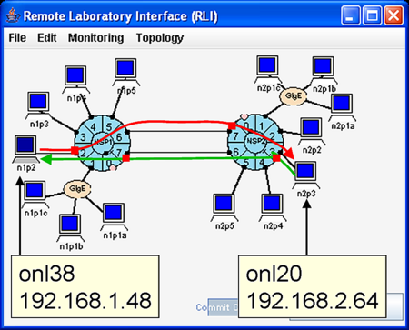
Consider again the example of sending ping traffic between n1p2 and n2p3 (Fig. 1). Initially, we will use the default routing tables so that ICMP echo request packets will travel left-to-right over the top link (1.6 to 2.7), and the returning ICMP echo reply packets will travel right-to-left over the bottom link (2.6 to 1.7). Then, we will demonstrate the effect on a traffic plot of changing the route table at port 2.3 so that reply packets travel right-to-left over the top link instead of over the bottom link.

Label Traffic Description (A) from 1.6 to 2.7 (B) from 1.2 to 1.6 (C) from 2.6 to 1.7 (D) from 1.7 to 1.2

Fig. 2. Monitoring Places.

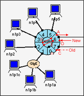
With default routing, the ICMP request packets will flow left-to-right over the top link (1.6 to 2.7), and the ICMP reply packets will flow right-to-left over the bottom link (2.6 to 1.7). The solid red circles in Fig. 2 indicate the approximate location of the places being monitored. The key concept is that the monitoring is being done inside the ATM switch component of the NSP router and not the FPX ports. This choice of monitoring points has implications which are explained in What Was Monitored In The Ping Example?.

Fig. 3. Monitoring Traffic From 1.6 to 2.7 (Menus).

In Fig. 3, we have selected NSP 1, Port 6 => Egress => Port Bandwidth to monitor the bandwidth leaving port 6. A dialogue box allows you to enter the monitoring period. For example, a period of 0.25 second means that the monitoring daemon will send out a control cell every 0.25 second to NSP 1's switch to read a byte counter and a clock counter which will be used to compute the traffic rate. Although most monitoring is done with a 1 second monitoring period (or longer), we have chosen 0.25 second here to highlight the moment when the packet is detected (i.e., the display will show spikes at 1 second intervals).

Fig. 4. Monitoring Traffic From 1.6 to 2.7 (Plot).

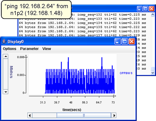
Fig. 4 shows the traffic display resulting from the ping command shown to the rear of the figure. The source of the ping traffic is n1p2 (192.168.1.48), and the destination is n2p3 (192.168.2.64). By default, the ping command sends a 64-byte (includes IP header) ICMP packet every second.

If this is the first monitoring display, a new display panel will appear. This panel will remain the focus of any additional monitoring points until you switch focus by either creating a new monitoring panel (Monitoring => Add Monitoring Display) or select Parameter => Add Parameter on an existing monitoring panel. As explained later, the default legend label on the right side of the display is OPPBW 6 which is the system's shorthand for Output Port Processor BandWidth 6.

Fig. 5. Monitoring Traffic From 1.2 to 1.6 (Menus).

A similar approach can be used to monitor the input bandwidth at port 2 going to port 6 (i.e., the traffic from 1.2 to 1.6) by selecting NSP 1, Port 2 => Ingress => Bandwidth to OPP to monitor the bandwidth from ingress port 2 going to egress port 6. But now the dialogue box will require not only the polling period (0.25 second) but also the output port destination (port 6 in this case). This second plot will be labeled IPP 2 BW to OPP 6 (i.e., the traffic going from the ATM switch's Input Port Processor 2 to Output Port Processor 5).

Fig. 6. Monitoring Traffic From 1.2 to 1.6 (Plot).

Fig. 6 shows all four desired traffic plots. The panel in the back is what you will see by default. The one in the front is the same panel but adusted to zoom into a smaller region of the display. This zoom feature will be discussed in a later page. In both panels, all four plots are almost identical as would be expected. The small variations between plots and variations over time are measurement artifacts that will be explained later.

Changing A Route Table

To show the effect of a route table change, we change the route table at NSP2/Port 3 so that returning ping traffic goes through link (2.7, 1.6) instead of (2.6, 1.7) (see Fig. 8).

Fig. 7. Changing the Reply Route (Menu).

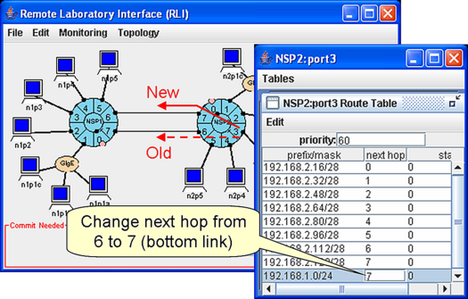
We modified the next hop for the prefix/mask 192.168.1.0/24 from 6 to 7 by clicking on the 6 and directly changing the value to 7. (An alternative approach would have been to add another route (NSP2:port3 Route Table =>Edit => Add Route) to port 7 with a longer matching prefix (e.g., 192.168.1.48/28) so that it took precedence over the route with prefix/mask of 192.168.1.0/24.)

Label Traffic Description Traffic Display Label (A) from 1.6 to 2.7 top right (B) from 1.2 to 1.6 1.2 to 1.6 (C) from 2.6 to 1.7 bottom left (D) from 2.7 to 1.6 top left (E) from 1.6 to 1.2 1.6 to 1.2

Fig. 8. Monitoring Places (Route Change).

Fig. 9. Changing the Reply Route (Plot).

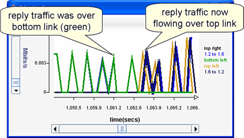
Fig. 9 shows that around 1,063 seconds the route table was modified so that the bottom left plot no longer shows any traffic while traffic has appeared in the top left and 1.6 to 1.2 plots.

We deleted the 1.7 to 1.2 plot from the original display, customized the labels and added two more plots (top left and 1.6 to 1.2). The display labels can be modified by selecting the label and changing the label shown in the dialogue box (described in the next page). The bottom two plots were added by following this recipe:

• top left: Select NSP1, Port 6 => Ingress => Port Bandwidth and fill out the dialogue box.
• 1.6 to 1.2: Select NSP1, Port 6 => Ingress => Bandwidth to OPP and fill out the dialogue box.

Tutorial >> The Remote Laboratory Interface	TOC