| Tutorial >> Filters, Queues and Bandwidth |
|
Packets arriving to an ingress Port are placed into separate Virtual Output Queues (VOQs) based on their forwarding port. Since each NSP has eight ports, there are eight VOQs at each input port. VOQ k contains packets that are to be forwarded to egress port k. The use of VOQs avoids the head-of-the-line (HOL) blocking problem that occurs when there is only a single queue. The page Tutorial => Filters, Queues and Bandwidth => NSP_Architecture => Queues describes in detail the NSP queues that are encountered as a packet travels from one host to another through an NSP.
We describe how the VOQs at ports 2.2 through 2.4 and port 1.7 of our two-NSP configuration can be monitored in a meaningful manner when there are three UDP flows. We also introduce the Add Formula dialogue box that allows us to define incremental bandwidth plots and other similar graphical compositions.
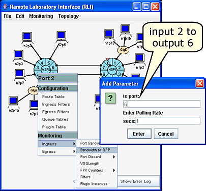
Fig. 1 shows the menus involved in monitoring the traffic volume passing through VOQ 6 at ingress port 2.2 (the left NSP). The recipe is:
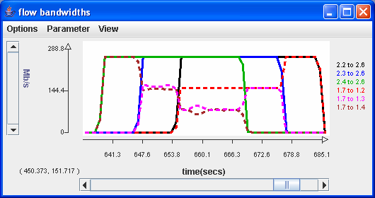
Fig. 2 shows the bandwidth chart of the following six UDP flows: 2.n-to-2.6 and 1.7-to-1.n for n=2, 3, 4. But this chart is difficult to read because most of the lines fall on top of each other.
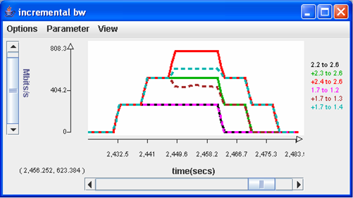
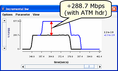
Fig. 3 shows plots which are easier to read because it shows the incremental bandwidths; i.e., the 2.3-to-2.6 bandwidth (labeled +2.3 to 2.6) is "stacked" on top of the 2.2-to-2.6 bandwidth, and the 2.4-to-2.6 bandwidth (labeled +2.4 to 2.6) is stacked on top of the 2.2-to-2.6 bandwidth. Similarly, the 1.7-to-1.n bandwidth lines are stacked on top of each other.
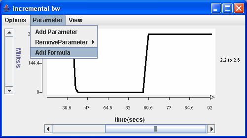
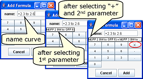
We now describe how to construct an incremental bandwidth chart. In Fig. 4, we laid down the base 2.2-to-2.6 plot in the standard manner. Now, we want to add two more lines each stacked on top of the previous line and then repeat the process for the 1.7-to-1.n lines.
The plot in Fig. 4 was created in the standard manner to lay the base 2.2-to-2.6 plot. In order to display the bandwidth in incremental format, we select the Parameter => Add Formula menu item in the display panel and the Add Formula dialogue box appears.
The Add Formula feature acts just like a calculator. Suppose that the three plots of 2.n-to-2.6 (n = 2, 3, 4) are represented by the three time series X[], Y[] and Z[] where X[] represents the sequence X[0], X[1], .... In effect, we would like to display X[i], X[i]+Y[i] and X[i]+Y[i]+Z[i] for i = 0, 1, 2, .... However, in our example, we visually indicate the time series by selecting the monitoring items instead of the time series X[], Y[] and Z[].
The recipe for creating the +2.3 to 2.6 plot (after the 2.2 to 2.6 plot) is:
| Window/Panel | Selection/Entry | Explanation |
|---|---|---|
| incremental bw | Parameter => Add Formula |
Open Add Formula panel |
| Add Formula | name: +2.3 to 2.6 | Enter the name (label) of the curve |
| Main RLI | Port 2/2 => Bandwidth to OPP | Opens Add Parameter window |
| Add Parameter | to port: 6 | VOQ (output port) number is 6. "M(2.2 to 2.6)" label appears on Add Formula panel |
| |
Enter Polling Rate 1 | 1 second polling rate |
| Add Formula | Select + button | We want to add another time series |
| Main RLI | Port 2/3 => Bandwidth to OPP | Opens Add Parameter window |
| Add Parameter | to port: 6 | VOQ (output port) number is 6. Label in Add Formula panel becomes "M(2.2 to 2.6)+M(2.3 to 2.6)" |
| |
Enter Polling Rate 1 | 1 second polling rate |
| Add Formula | Select Add button | Add formula to the incremental bw chart |
The traffic chart will look like Fig. 6 below.
We repeat the above procedure to add the other incremental bandwidth plots. Note that when we setup the +2.4 to 2.6 plot we will have to specify three monitoring points: the Bandwidth to OPP (VOQ bandwidth) for the three traffic bandwidths flowing from 2.n to 2.6 (n=1, 2, 3). The result will be Fig. 3.
Revised: Fri, July 21, 2006
| Tutorial >> Filters, Queues and Bandwidth |
|