ONL Tutorial

The ONL Tutorial

Tutorial >> Filters, Queues and Bandwidth

TOC

Mapping Flows to Separate Queues

Instead of mapping all three UDP flows to queue 300 at egress port 2.6, we could map them to separate queues so that we can give guaranteed bandwidth to each flow. We will still use the Queue Table to define the packet scheduling characteristics, but now, we will map each of the three UDP flows to each of the queues 300-302.

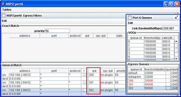
Fig. 1. Mapping Flows to Queues 300, 301 and 302.

In Fig. 1, the qid fields in the Egress Filters table have been changed so that the packets from n2p3 and n2p4 will now go to queues 301 and 302 respectively instead of queue 300. And, entries for queues 300-302 have been added to the Port 6 Queues table (select Tables => Queue Table in the NSP2:port6 window to show the table). The packet scheduling parameters for queues 300-302 have been chosen so that the packet discard thresholds are different (30,000, 40,000, 50,000) but the quantum fields are the same (2,048).

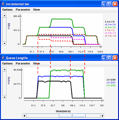
Fig. 2. Incremental Bandwidth and Queue Length Charts.

Fig. 2 shows the effect on the incremental bw traffic chart and the Queue Lengths chart. Because the quantum parameter for all three queues are all equal to 2,048, they will all get an equal share of the link bandwidth. But because the threshold parameters are in the ratio 3:4:5, their maximum queue lengths will be in that ratio with the largest queue topping out at 50,000 bytes.

Unequal Bandwidth Shares

Fig. 3. Port 2.6 Queue Table.

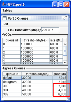
Fig. 3 shows the new Queue Table where we have changed the quantum parameters for queues 300-302 so that the bandwidth shares of these queues are now in the approximate ratio of 1:2:3. Now, queue 301 should get about twice as much bandwidth as queue 300, and queue 302 should get about 1.5 as much bandwidth as queue 301 under full load.

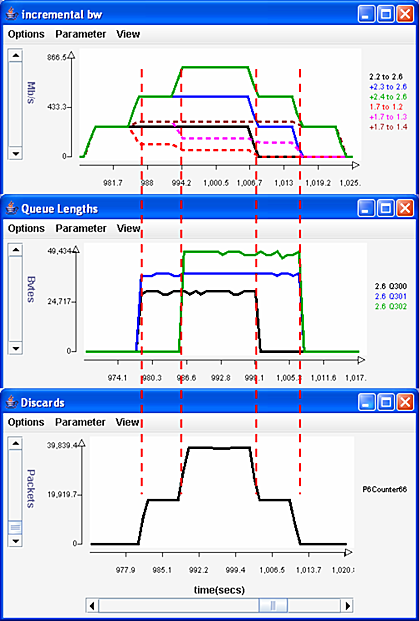
Fig. 4. Effect of Greater Share to Queue 302.

Fig. 4 shows the effect of these changes on the bandwidth, queues and discards. The five time periods exhibit the expected bandwidth behavior:

Before T=986: Since n2p2-n1p2 is the only flow active, it gets the entire link bandwidth and transmits at 250 Mbps; there is no queueing; and there are no packet discards.
Between T=986 and T=994: Now flow n2p3-n1p3 joins in and there are two competing flows with an aggregate demand of 500 Mbps which is 200 Mbps over the 300 Mbps link bandwidth. The incremental bandwidth chart shows the bandwidth ratio for these two flows is 1:2; i.e., queue 300 gets 100 Mbps, and queue 301 gets 200 Mbps. Because the link is over subscribed, backlogs develop for both queue 300 and 301, and packets are discarded.
Between T=994 and T=1,008: Flow n2p4-n1p4 becomes active, and there are three competing flows with an aggregate demand of 750 Mbps which is 450 Mbps over the 300 Mbps link bandwidth. The incremental bandwidth chart shows the bandwidth ratios for the three flows is 1:2:3; i.e., queue 300 gets 50 Mbps, queue 301 gets 100 Mbps, and queue 302 gets 150 Mbps. Because the link is still over subscribed, there are still backlogs at all three queues, and packets are discarded.
Between T=1,008 and T=1,015: The two flows n2p3-n1p3 and n2p4-n1p4 are active and share the bottleneck link in a 2:3 ratio (i.e., 120 Mbps and 180 Mbps).
After T=1,015: Since only the n2p4-n1p4 flow is active, all of its 250 Mbps traffic is transmitted through the bottleneck link.

During the periods of congestion, the Discards chart is nearly identical to the ones described in the page Mapping Flows to a Single Queue since the only difference is that the flows are mapped to separate queues. That is, since the excess input traffic rate is the same as before, and the only difference is that the total amount of buffering here is less than before, the only difference should be that the onset of packet drops is earlier than before (which is hard to see in the chart).

Using Exact Match Filters

Exact Match (EM) filters can also be used in a similar manner as GM filters. We will use an EM filter to override the GM filter associated with queue 300. But when using EM filters with UDP flows, we need to know all IP header fields in the filter which will require that we use the Unix netstat command.

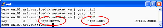
Fig. 5. Port Numbers From the netstat Command.

Fig. 5 shows how to use the netstat command to determine the port number fields in the EM filter. The command netstat -a displays all of the listening and non-listening sockets, and grep n2p2 grabs only those lines containing the string n2p2 which is the name of the iperf client host. The output here shows that the client is using port 32784 (an ephemeral port assigned by n2p2's operating system) and the server is using port 5001 (the default iperf server port).

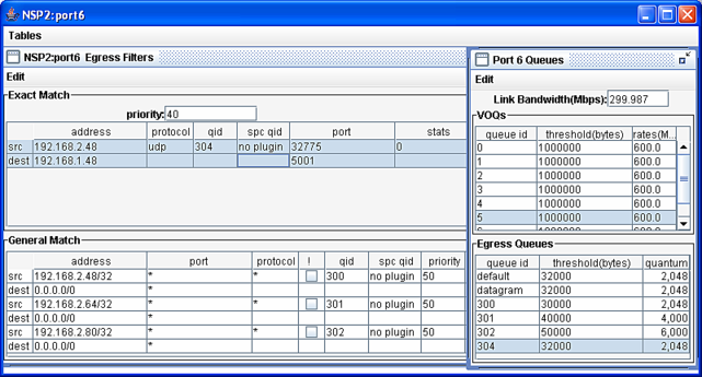
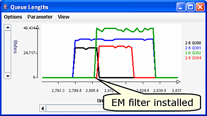
Fig. 6. High Priority Exact Match Filter.

Fig. 6 shows that we have added an EM filter that will send packets from n1p2 (192.168.2.48) to queue 304. The first GM filter will also match UDP packets from n1p2, but its priority (50) is lower than the EM filter priority of 40 (a lower priority number indicates a higher priority). Fig. 7 shows that queue 304 (2.6 Q304 line) is now getting a backlog, but queue 300 (2.6 Q300 line) no longer has a backlog.

Fig. 7. Effect of EM Filter on Queue Length Chart.

Revised: Mon, July 31, 2006

Tutorial >> Filters, Queues and Bandwidth	TOC